[1] "Timestamp"
[2] "Email Address"
[3] "Which days of the bootcamp will you attend?"
[4] "What is your name?"
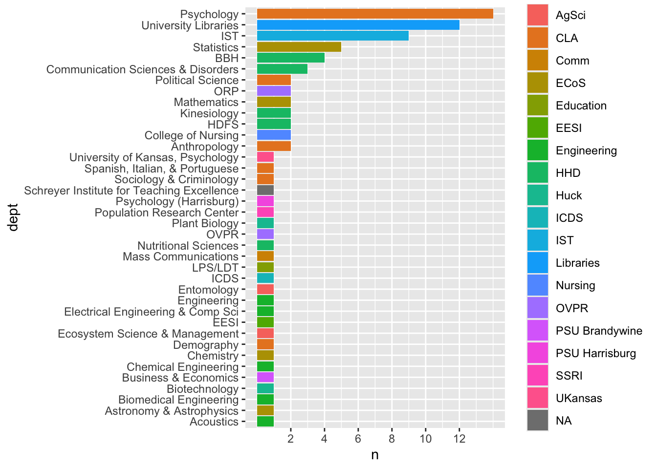
[5] "What is your department or unit?"
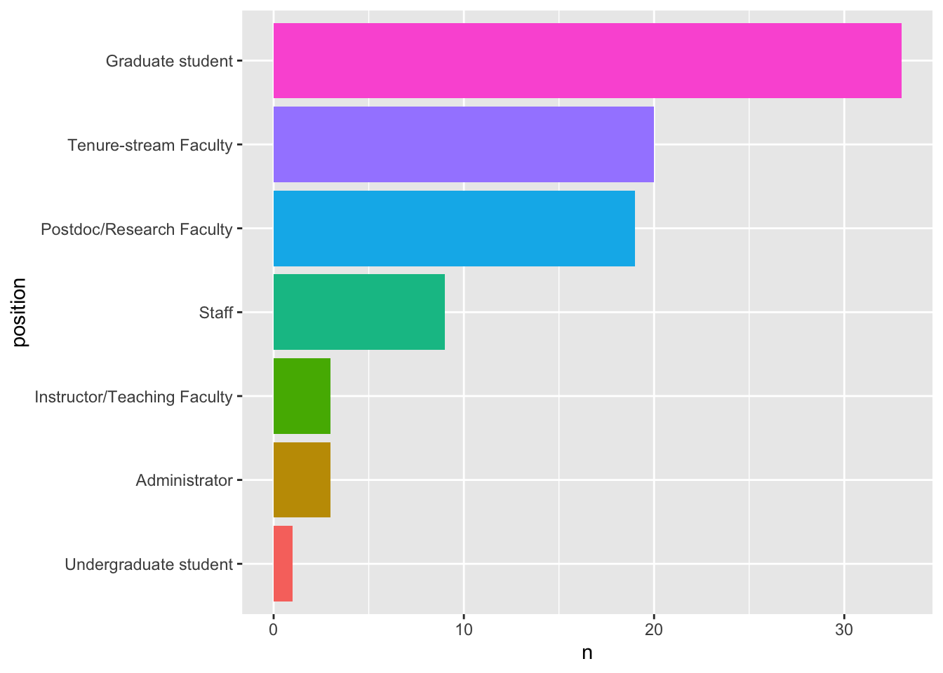
[6] "What is your current position?"
[7] "Any comments?"
[8] "Are you interested in registering for the 2.5 day bootcamp or the Keynote address(es)?"
[9] "Which Keynote address(es) are you interested in attending?"
[10] "presenter"
Google Forms conveniently returns the questions as variable names at the top of each column. These are handy for creating a data dictionary, but awkward for data processing. We rename these for our convenience. We also export a data dictionary.
Code
reqistrations_qs <-names(registrations)registrations_clean <- registrations |> dplyr::rename(timestamp ="Timestamp",attend_days ="Which days of the bootcamp will you attend?",name ="What is your name?",psu_email ="Email Address",dept ="What is your department or unit?",position ="What is your current position?",comments ="Any comments?",bootcamp_keynote ="Are you interested in registering for the 2.5 day bootcamp or the Keynote address(es)?",which_keynotes ="Which Keynote address(es) are you interested in attending?" )registrations_short <-c("timestamp","psu_email","attend_days","name","dept","position","bootcamp_keynote","which_keynotes","comments","presenter")registrations_pid <-c(FALSE, FALSE, FALSE, TRUE, FALSE, FALSE, FALSE, FALSE, FALSE, FALSE)registrations_dd <-data.frame(qs = reqistrations_qs, qs_short = registrations_short, pid = registrations_pid)registrations_dd |> knitr::kable(format ='html')readr::write_csv(registrations_dd,file =file.path(params$csv_dir, "registrations-2025-data-dict.csv"))
Table 10.1: A minimal data dictionary.
qs
qs_short
pid
Timestamp
timestamp
FALSE
Email Address
psu_email
FALSE
Which days of the bootcamp will you attend?
attend_days
FALSE
What is your name?
name
TRUE
What is your department or unit?
dept
FALSE
What is your current position?
position
FALSE
Any comments?
bootcamp_keynote
FALSE
Are you interested in registering for the 2.5 day bootcamp or the Keynote address(es)?
which_keynotes
FALSE
Which Keynote address(es) are you interested in attending?
registrations_yes <- registrations_yes |> dplyr::mutate(dept = dplyr::recode( dept,`Clinical Psychology`="Psychology",`Psychology (Cognitive)`="Psychology",`Psychology / SSRI`="Psychology",`Department of Psychology`="Psychology",`Cognitive Psychology`="Psychology",`Psychology, Developmental`="Psychology",`Developmental Psychology (CAT Lab)`="Psychology",`Developmental Psychology`="Psychology",`Psych`="Psychology",`English language`="English",`english`="English",`English Language Teaching`="English",`English Department`="English",`Languages`="Global Languages & Literatures",`Languages and Literature`="Global Languages & Literatures",`Department of Foreign Languages`="Global Languages & Literatures",`Linguistics`="Applied Linguistics",`Department of Sociology and Criminology`="Sociology & Criminology",`Communication Sciences and Disorders`="Communication Sciences & Disorders",`CSD`="Communication Sciences & Disorders",`Human Development and Family Studies & Social Data Analytics`="HDFS",`Human Development and Family Studies`="HDFS",`Human Development and Family Studies (HDFS)`="HDFS",`Department of Human Development and Family Studies`="HDFS",`Human Development and Family Sciences`="HDFS",`HDFS/DEMO`="HDFS",`bbh`="BBH",`Biobehavioral Health`="BBH",`Biobehavioural Health`="BBH",`Biobehavioural Health`="BBH",`Biobehavioral health`="BBH",`RPTM`="Recreation, Park, & Tourism Management",`Sociology and Social Data Analytics`="Sociology",`Spanish Italian and portuguese`="Spanish, Italian, & Portuguese",`Spanish, Italian, and Portuguese Department`="Spanish, Italian, & Portuguese",`Spanish Italian and Portuguese`="Spanish, Italian, & Portuguese",`Spanish, Italian, and Portuguese`="Spanish, Italian, & Portuguese",`French and Francophone Studies`="French & Francophone Studies",`DEMOG`="Demography",`Nutrition`="Nutritional Sciences",`College of IST`="IST",`Statistics Department`="Statistics",`Department of Statistics`="Statistics",`Math`="Mathematics", `Astronomy and Astrophysics`="Astronomy & Astrophysics",`Recreation, Park and Tourism Management`="Recreation, Park, & Tourism Management",`SHS`="Student Health Svcs",`Department of Chemical Engineering`="Chemical Engineering",`ESM`="Engineering Science & Mechanics",`Engineering Science`="Engineering Science & Mechanics",`Engineering Science and Mechanics`="Engineering Science & Mechanics",`EECS`="Electrical Engineering & Comp Sci",`Department of Food Science`="Food Science",`Libraries`="University Libraries",`University libraries`="University Libraries",`Ecosystem Science and Management`="Ecosystem Science & Management",`PRC`="Population Research Center",`TLT, PSU Libraries`="University Libraries",`Business and Economics`="Business & Economics",`EE`="Electrical Engineering",`College of Medicine / Clinical and Translational Science Institute`="CTSI",`Mechanical engineering,Penn state Harrisburg`="Mechanical Engineering (Harrisburg)",`Smeal College of Business, Accounting`="Accounting",`School of Science, Engineering, and Technology`="Sci, Engr, & Tech" ) ) |> dplyr::mutate(college =case_match( dept,"Statistics"~"ECoS","University of Kansas, Psychology"~"UKansas","Biology"~"ECoS","Psychology"~"CLA","Spanish, Italian, & Portuguese"~"CLA","Research Informatics and Publishing"~"Libraries","Political Science"~"CLA","Applied Linguistics"~"CLA","Global Languages & Literatures"~"CLA","Anthropology"~"CLA","Sociology"~"CLA","English"~"CLA","C-SoDA"~"CLA","Office of Digital Pedagogies and Initiatives"~"CLA","Asian Studies"~"CLA","Sociology & Criminology"~"CLA","IST"~"IST","Chemical Engineering"~"Engineering","Material Science and Engineering"~"Engineering","Engineering Science & Mechanics"~"Engineering","College of Engineering"~"Engineering","Biomedical Engineering"~"Engineering","Nutritional Sciences"~"HHD","HDFS"~"HHD","Kinesiology"~"HHD","Recreation, Park, & Tourism Management"~"HHD","BBH"~"HHD","College of Nursing"~"Nursing","Bellisario College of Communication"~"Comm","Mass Communications"~"Comm","Marketing"~"Smeal","Food Science"~"Ag","Neuroscience"~"Med","College of Human and Health Development"~"HHD","University Libraries"~"Libraries","ICDS"~"ICDS","EESI"~"EESI","ORP"~"OVPR","Astronomy & Astrophysics"~"ECoS","Chemistry"~"ECoS","Mathematics"~"ECoS","Entomology"~"AgSci","Ecosystem Science & Management"~"AgSci","Plant Biology"~"Huck","Biotechnology"~"Huck","Acoustics"~"Engineering","Communication Sciences & Disorders"~"HHD","Electrical Engineering & Comp Sci"~"Engineering","Population Research Center"~"SSRI","Psychology (Harrisburg)"~"PSU Harrisburg","Business & Economics"~"PSU Brandywine","Engineering"~"Engineering","LPS/LDT"~"Education","Demography"~"CLA","OVPR"~"OVPR","Mechanical Engineering"~"Engineering","Electrical Engineering"~"Engineering","Medicine"~"Medicine","CTSI"~"Medicine","French & Francophone Studies"~"CLA","Data Analytics"~"IST","Cybersecurity"~"IST","Mechanical Engineering (Harrisburg)"~"PSU Harrisburg","Accounting"~"Smeal","PSU Harrisburg"~"PSU Harrisburg","Sci, Engr, & Tech"~"PSU Harrisburg","Schreyer Institute for Teaching Excellence"~"Old Main","HHD"~"HHD" ),.default ="Unknown",.missing ="Unknown" )